5.7 KiB
Apply Net
apply_net is a tool to print or visualize DensePose results on a set of images.
It has two modes: dump to save DensePose model results to a pickle file
and show to visualize them on images.
Dump Mode
The general command form is:
python apply_net.py dump [-h] [-v] [--output <dump_file>] <config> <model> <input>
There are three mandatory arguments:
<config>, configuration file for a given model;<model>, model file with trained parameters<input>, input image file name, pattern or folder
One can additionally provide --output argument to define the output file name,
which defaults to output.pkl.
Examples:
- Dump results of a DensePose model with ResNet-50 FPN backbone for images
in a folder
imagesto filedump.pkl:
python apply_net.py dump configs/densepose_rcnn_R_50_FPN_s1x.yaml DensePose_ResNet50_FPN_s1x-e2e.pkl images --output dump.pkl -v
- Dump results of a DensePose model with ResNet-50 FPN backbone for images
with file name matching a pattern
image*.jpgto fileresults.pkl:
python apply_net.py dump configs/densepose_rcnn_R_50_FPN_s1x.yaml DensePose_ResNet50_FPN_s1x-e2e.pkl "image*.jpg" --output results.pkl -v
If you want to load the pickle file generated by the above command:
# make sure DensePose is in your PYTHONPATH, or use the following line to add it:
sys.path.append("/your_detectron2_path/detectron2_repo/projects/DensePose/")

f = open('/your_result_path/results.pkl', 'rb')
data = pickle.load(f)
The file results.pkl contains the list of results per image, for each image the result is a dictionary:
data: [{'file_name': '/your_path/image1.jpg',
        'scores': tensor([0.9884]),
        'pred_boxes_XYXY': tensor([[ 69.6114,   0.0000, 706.9797, 706.0000]]),
        'pred_densepose': <densepose.structures.DensePoseResult object at 0x7f791b312470>},
       {'file_name': '/your_path/image2.jpg',
        'scores': tensor([0.9999, 0.5373, 0.3991]),
        'pred_boxes_XYXY': tensor([[ 59.5734,   7.7535, 579.9311, 932.3619],
                                   [612.9418, 686.1254, 612.9999, 704.6053],
                                   [164.5081, 407.4034, 598.3944, 920.4266]]),
        'pred_densepose': <densepose.structures.DensePoseResult object at 0x7f7071229be0>}]
We can use the following code, to parse the outputs of the first detected instance on the first image.
from densepose.data.structures import DensePoseResult
img_id, instance_id = 0, 0  # Look at the first image and the first detected instance
bbox_xyxy = data[img_id]['pred_boxes_XYXY'][instance_id]
result_encoded = data[img_id]['pred_densepose'].results[instance_id]
iuv_arr = DensePoseResult.decode_png_data(*result_encoded)
The array bbox_xyxy contains (x0, y0, x1, y1) of the bounding box.
The shape of iuv_arr is [3, H, W], where (H, W) is the shape of the bounding box.
iuv_arr[0,:,:]: The patch index of image points, indicating which of the 24 surface patches the point is on.iuv_arr[1,:,:]: The U-coordinate value of image points.iuv_arr[2,:,:]: The V-coordinate value of image points.
Visualization Mode
The general command form is:
python apply_net.py show [-h] [-v] [--min_score <score>] [--nms_thresh <threshold>] [--output <image_file>] <config> <model> <input> <visualizations>
There are four mandatory arguments:
<config>, configuration file for a given model;<model>, model file with trained parameters<input>, input image file name, pattern or folder<visualizations>, visualizations specifier; currently available visualizations are:bbox- bounding boxes of detected persons;dp_segm- segmentation masks for detected persons;dp_u- each body part is colored according to the estimated values of the U coordinate in part parameterization;dp_v- each body part is colored according to the estimated values of the V coordinate in part parameterization;dp_contour- plots contours with color-coded U and V coordinates
One can additionally provide the following optional arguments:
--min_scoreto only show detections with sufficient scores that are not lower than provided value--nms_threshto additionally apply non-maximum suppression to detections at a given threshold--outputto define visualization file name template, which defaults tooutput.png. To distinguish output file names for different images, the tool appends 1-based entry index, e.g. output.0001.png, output.0002.png, etc...
The following examples show how to output results of a DensePose model
with ResNet-50 FPN backbone using different visualizations for image image.jpg:
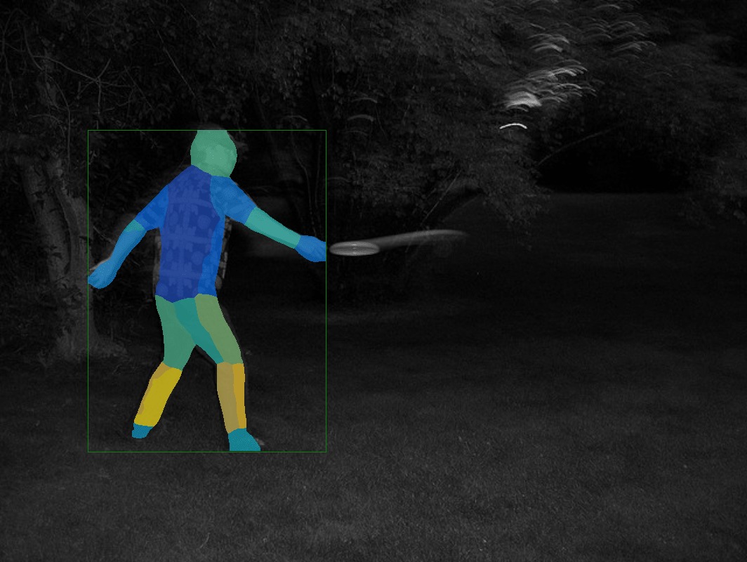
- Show bounding box and segmentation:
python apply_net.py show configs/densepose_rcnn_R_50_FPN_s1x.yaml DensePose_ResNet50_FPN_s1x-e2e.pkl image.jpg bbox,dp_segm -v
- Show bounding box and estimated U coordinates for body parts:
python apply_net.py show configs/densepose_rcnn_R_50_FPN_s1x.yaml DensePose_ResNet50_FPN_s1x-e2e.pkl image.jpg bbox,dp_u -v

- Show bounding box and estimated V coordinates for body parts:
python apply_net.py show configs/densepose_rcnn_R_50_FPN_s1x.yaml DensePose_ResNet50_FPN_s1x-e2e.pkl image.jpg bbox,dp_v -v

- Show bounding box and estimated U and V coordinates via contour plots:
python apply_net.py show configs/densepose_rcnn_R_50_FPN_s1x.yaml DensePose_ResNet50_FPN_s1x-e2e.pkl image.jpg dp_contour,bbox -v
