# Analysis tools
<!-- TOC -->
- [Analysis tools](#analysis-tools)
- [Count number of parameters](#count-number-of-parameters)
- [Publish a model](#publish-a-model)
- [Reproducibility](#reproducibility)
- [Log Analysis](#log-analysis)
- [Visualize Datasets](#visualize-datasets)
- [Use t-SNE](#use-t-sne)
## Count number of parameters
```shell
python tools/analysis_tools/count_parameters.py ${CONFIG_FILE}
```
An example:
```shell
python tools/analysis_tools/count_parameters.py configs/selfsup/mocov2/mocov2_resnet50_8xb32-coslr-200e_in1k.py
```
## Publish a model
Before you publish a model, you may want to
- Convert model weights to CPU tensors.
- Delete the optimizer states.
- Compute the hash of the checkpoint file and append the hash id to the filename.
```shell
python tools/model_converters/publish_model.py ${INPUT_FILENAME} ${OUTPUT_FILENAME}
```
An example:
```shell
python tools/model_converters/publish_model.py YOUR/PATH/epoch_100.pth YOUR/PATH/epoch_100_output.pth
```
## Reproducibility
If you want to make your performance exactly reproducible, please set `--cfg-options randomness.deterministic=True` to train the final model. Note that this will switch off `torch.backends.cudnn.benchmark` and slow down the training speed.
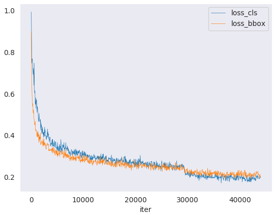
## Log Analysis
`tools/analysis_tools/analyze_logs.py` plots loss/lr curves given a training
log file. Run `pip install seaborn` first to install the dependency.
```shell
python tools/analysis_tools/analyze_logs.py plot_curve [--keys ${KEYS}] [--title ${TITLE}] [--legend ${LEGEND}] [--backend ${BACKEND}] [--style ${STYLE}] [--out ${OUT_FILE}]
```
Examples:
- Plot the classification loss of some run.
```shell
python tools/analysis_tools/analyze_logs.py plot_curve log.json --keys loss_dense --legend loss_dense
```
- Plot the classification and regression loss of some run, and save the figure to a pdf.
```shell
python tools/analysis_tools/analyze_logs.py plot_curve log.json --keys loss_dense loss_single --out losses.pdf
```
- Compare the loss of two runs in the same figure.
```shell
python tools/analysis_tools/analyze_logs.py plot_curve log1.json log2.json --keys loss --legend run1 run2
```
- Compute the average training speed.
```shell
python tools/analysis_tools/analyze_logs.py cal_train_time log.json [--include-outliers]
```
The output is expected to be like the following.
```text
-----Analyze train time of work_dirs/some_exp/20190611_192040.log.json-----
slowest epoch 11, average time is 1.2024
fastest epoch 1, average time is 1.1909
time std over epochs is 0.0028
average iter time: 1.1959 s/iter
```
## Visualize Datasets
`tools/misc/browse_dataset.py` helps the user to browse a mmselfsup dataset (transformed images) visually, or save the image to a designated directory.
```shell
python tools/misc/browse_dataset.py ${CONFIG} [-h] [--skip-type ${SKIP_TYPE[SKIP_TYPE...]}] [--output-dir ${OUTPUT_DIR}] [--not-show] [--show-interval ${SHOW_INTERVAL}]
```
An example:
```shell
python tools/misc/browse_dataset.py configs/selfsup/simsiam/simsiam_resnet50_8xb32-coslr-100e_in1k.py
```
## Use t-SNE
We provide an off-the-shelf tool to visualize the quality of image representations by t-SNE.
```shell
python tools/analysis_tools/visualize_tsne.py ${CONFIG_FILE} --checkpoint ${CKPT_PATH} --work-dir ${WORK_DIR} [optional arguments]
```
Arguments:
- `CONFIG_FILE`: config file for the pre-trained model.
- `CKPT_PATH`: the path of model's checkpoint.
- `WORK_DIR`: the directory to save the results of visualization.
- `[optional arguments]`: for optional arguments, you can refer to [visualize_tsne.py](https://github.com/open-mmlab/mmselfsup/blob/master/tools/analysis_tools/visualize_tsne.py)
An example:
```shell
python tools/analysis_tools/visualize_tsne.py configs/selfsup/simsiam/simsiam_resnet50_8xb32-coslr-100e_in1k.py --checkpoint epoch_100.pth --work-dir work_dirs/selfsup/simsiam_resnet50_8xb32-coslr-200e_in1k
```